Methods notes on the use of disease risks in STAPM
Methods_for_STAPM_disease_risks.RmdBackground
Tobacco and alcohol are leading causes of preventable disease and of socio-demographic inequalities in health and there is a great deal of literature that reports estimates of the relationship between tobacco or alcohol consumption and the risk of having or dying from a wide range of conditions. There is less information available to estimate how tobacco and alcohol consumption might combine to influence disease risk, and so for STAPM we needed to collate and understand the available information.
This vignette describes how we use the relative risks of disease in STAPM, written as a guide to help understand the functions in the tobalcepi package.
Approach taken to develop the tobalcepi package
Literature reviewing
The list of diseases, their ICD-10 code definitions and the associated risk functions were collated from periodic reviews of the literature, drawing primarily on other existing reviews. See these technical reports for further information:
- Alcohol and disease risks report (Angus et al. 2018).
- Smoking and disease risks report (Webster et al. 2018).
R functions to assign relative risks of disease to individuals
To organise the information on the relative risks of diseases due to tobacco and alcohol consumption, and to provide functions to easily work with these data in modelling, we built the tobalcepi R code package (click on the link to the package webpage for introductory information). The R code functions are version controlled so that each project works with a specified version of the package (see the version tracking sheet), and error-fixes and new developments can be tracked (see the issues log and software development tasks tracking sheet.
The function tobalcepi::RRFunc() does the job of
assigning the relative risks of each disease to a sample of individuals
according to their current alcohol and/or tobacco consumption status.
tobalcepi::RRFunc() has options that can tailor it to
assign risks based on tobacco consumption only, alcohol consumption
only, or both tobacco and alcohol consumption.
Example calculations using functions from the tobalcepi package
To illustrate the use of the tobalcepi functions for
different tasks, we have begun to create example workflows. You can use
these examples to help understand how the code works, run them to
generate model inputs, or use them as a starting point for the
development of a new project (at the moment, these workflows are
accessible only to the project team).
The workflows are listed below:
- Population attributable fractions. Working code repository for the estimation and exploration of the fractions of disease attributable to tobacco and/or alcohol.
Alcohol related risks of disease
See the alcohol and disease risks report (Angus et al. 2018). The alcohol modelling considers 45 categories of adult diseases related to alcohol consumption and the corresponding dose-response effects of current levels of alcohol consumption on the relative risks of disease. The model links average weekly alcohol consumption to the risk of chronic diseases, and the amount of alcohol consumed on single drinking occasions to health harms associated with intoxication.
“Partial acute” alcohol risk functions
Here we describe the approach taken in STAPM to model the health harms that are partially-attributable to level of acute alcohol intake on a single occasion (i.e. related to intoxication). The health harms that we consider could be intentional or unintentional, e.g. traffic accidents, assault or falls. “Partially-attributable acute” means that the harm can occur without alcohol but the risk of occurrence changes with intoxication.
We build on the method used to model the health harms due to intoxication in the Sheffield Alcohol Policy Model (SAPM). The methods used for this module of SAPM have evolved over time. Originally, the risk of harm was inferred from external information on the alcohol attributable fractions of traffic accidents, assaults, falls etc. (described in the Purshouse et al. modelling report for NICE (2009)). The method was updated to allow SAPM to model individual exposure to the risk of harm from each drinking occasion, e.g. for how long is someone intoxicated after drinking and what is their risk of a fall injury when intoxicated – this new method is described in two papers by Hill-McManus et al. (2014; 2014). Most recently, the method was updated to incorporate new estimates of the risk of health harms due to intoxication by Cherpitel et al. (2015) – these are described in the alcohol risk functions report (Angus et al. 2018).
The latest SAPM method
Number of drinking occassions
The first step is to estimate the number of drinking occasions that an individual has in a year and we have two sources of information on this.
Source of information 1. The HSE asks repondents about the
frequency they drank alcoholic drinks in the last 12 months (in the
variable dnoft), offering the responses: Almost every day,
Five or six days a week, Three or four days a week, Once or twice a
week, Once or twice a month, Once every couple of months, Once or twice
a year. For interval frequencies, we take the mid point value. We
convert yearly frequencies to weekly frequency. For example, Three or
four days a week becomes 3.5 times a week. This processing is done by
the function hseclean::alc_drink_now_allages() that calls
the function hseclean::alc_drink_freq().
Source of information 2. Hill-McManus et al. (2014) developed a method to estimate the
number of drinking occasions per year using data from detailed diaries
in the National Diet and Nutrition Survey (NDNS) 2000/2001. Using the
regression coefficients from this study, it is possible to predict each
individual’s expected number of drinking occasions across the year, the
average amount they drunk on an occasion, the variability in the amount
drunk among occasions, and how these vary socio-demographically.
Hill-McManus et al. use a negative binomial regression model for the
number of weekly drinking occasions (see their Table 3). The explanatory
variables for the number of weekly drinking occasions were: log weekly
mean consumption, age, income (in poverty or not), ethnicity
(white/non-white), age left education, number of children, social class
(manual/non-manual). From the regression coefficients we calculate the
expected number of weekly drinking occasions for each individual in the
HSE data (implemented in the STAPM code by the function
tobalcepi::AlcBinge()). Note that this model was fitted to
a population sample aged below 65 years, but we assume the effect at
55–65 years applies at older ages too.
Amount drunk on drinking occasions
The second step is to estimate the distribution of the amounts that each individual drinks on their drinking occasions. The HSE does not provide this information – it asks questions on the number of units that each individual drank on their heaviest drinking day in the last seven days but this does not tell us about the distribution of amounts drunk across all drinking occasions in a year.
SAPM uses the method developed by Hill-McManus et al. (2014) – there are two parts to the process of estimating the distribution of amount drunk.
First, estimate the average quantity of alcohol that we expect each individual to consume on a drinking occasion. Hill-McManus et al. estimated regression coefficients (their Table 4) that allow predictions of the average amount consumed. The predictors of average amount consumed were: log weekly mean consumption, age, sex, ethnicity (non-white/white), and an interaction between sex and log weekly mean consumption (indicating that men and women differ in the number of drinking occasions required to achieve the same level of weekly consumption). Note that an estimate of the average quantity of alcohol consumed on a drinking occasion can also be obtained from the HSE data by dividing average weekly consumption by the number of weekly drinking occasions.
Second, estimate the individual-level variability in the amount consumed across their drinking occasions. To do this, Hill-McManus et al. fitted two Heckman regression models to the NDNS data:
Model 1 was a Heckman selection model designed to correct the analysis for the problem that the NDNS data only provides a seven-day snapshot of each individual’s annual drinking, and at least three data points per individual are needed to estimate the variability in amount drunk. The Heckman selection model estimated the probability that an individual drank on at least three separate occasions during the diary period (see their Table 5). The results were used to correct the estimates of variability for selection bias via the Inverse Mills Ratio. The predictors of an individual drinking on at least three separate occasions during the diary period were: log weekly mean consumption, age, income (in poverty or not), employed/not-employed, ethnicity (non-white/white), age left education, number of children, social class (manual/non-manual).
Model 2 was a Heckman outcome regression fitted to the standard deviation of the quantity of alcohol consumed in a drinking occasion (see their Table 6). The predictors of the standard deviation in the quantity of alcohol consumed in a drinking occasion were: log weekly mean consumption, income (in poverty or not), and the Inverse Mills ratio.
In the STAPM code, the function tobalcepi::AlcBinge()
uses the HSE data and the regression coefficients from Hill-McManus et
al. to infer the mean and standard deviation of amount drunk on each
drinking occasion by individuals who drink. From these two parameters,
we then calculate individual-specific probability density functions of
the amount of alcohol consumed on a drinking occasion (in the STAPM
code, this is done within the function
tobalcepi::PArisk()).
Time spent intoxicated
The third step is to estimate each individual’s annual exposure to the risk of health harms due to intoxication, as defined by the amount of time that they spend intoxicated during a year (here we use ‘intoxicated’ to mean having a percentage blood alcohol content (%BAC) greater than zero). The method that we use to estimate the time that each individual spends intoxicated over a year is described in Hill-McManus et al. (2014), who drew on Taylor et al. (2011).
The expected duration of intoxication for each amount of alcohol drunk on an occassion is defined in terms of the time, in hours, after a drinking occasion that it would take for an individual’s %BAC to drop to zero. The calculation of this time considers:
an individual’s sex, height and weight;
Widmark’s \(r\) (the fraction of the body mass in which alcohol would be present if it were distributed at concentrations equal to that in blood - see examples of use of the Widmark equation in Watson (1981) and Posey and Mozayani (2007));
the rate at which the liver clears alcohol from the body (we assume this is 0.017 %BAC per hour).
To simplify the calculation, we do not consider the rate of alcohol absorption (i.e. there is no alcohol absorption rate constant) or the time interval between drinks within a drinking occasion.
The calculation of the time that each individual spends intoxicated
in a year multiplies the probability that each level of alcohol is
consumed on a drinking occasion by the expected duration of intoxication
for each amount of alcohol that could be drunk on an occasion. This is
then multiplied by the expected number of drinking occasions per week
and by 52 weeks in a year. Finally, the time spent intoxicated is summed
to give the expected time spent intoxicated in a year (in the STAPM
code, this is implemented by the function
tobalcepi::PArisk()).
The annual relative risk of partially-attributable acute conditions
The relative risks for alcohol-related injuries are taken from Cherpitel et al. (2015) and described in our alcohol risk functions report (Angus et al. 2018). Note that Cherpitel et al. report relative risks by the number of standard drinks consumed (we assume 1 Std. drink = 16ml (12.8g) of ethanol). The risk functions in Cherpital differ by four causes of health harm, which we map onto our disease list as follows:
- Traffic
- Violence: “Assault”, “Other_intentional_injuries”
- Falls
- Other: “Mechanical_forces”, “Drowning”, “Other_unintentional_injuries”, “intentional_self_harm”, “Accidental_poisoning”, “Fire_injuries”.
To calculate the annual relative risk for each condition, we do the following:
match each amount drunk on a drinking occasion to the associated relative risk (e.g. the relative risk of violence after a drinking occasion where 6 standard drinks were consumed);
multiply the relative risk associated with each drinking occasion by the expected amount of time spent intoxicated following that drinking occasion;
sum the relative risk associated with the time during the year that is spent intoxicated (the remaining time in the year that is not spent intoxicated has a relative risk of 1).
The final estimate of each individual’s annual relative risk of a
partially-attributable acute condition is the average risk considering
time spent intoxicated and time not spent intoxicated (in the STAPM code
the calculations are implemented by the function
tobalcepi::PArisk()).
Adaptation to suit STAPM
The problem
STAPM uses a different method of modelling to SAPM in that STAPM tracks
individuals as they age (the within-cohort dynamics) but SAPM does not –
instead SAPM models changes over time (in one-year time steps) to
repeated cross-sectional samples of individuals from the HSE. The method
described above is easily applied to a sample of individuals from the
HSE (the SAPM method), because the HSE contains the necessary covariate
(i.e. in the HSE sample there is also data on ethnicity, income, number
of children etc.). For STAPM to use the method, would require it to also
track the individual age trajectories of traits such as income – and
this is beyond the current scope of the STAPM modelling.
The solution
The STAPM modelling tracks the individual age trajectories of the
average weekly amount of alcohol consumed – the dynamics of these
trajectories are stratified by sex and Index of Multiple Deprivation
(IMD) quintiles. We therefore need to adapt the method to predict the
number of drinking occasions and the distribution of amount consumed as
a function of the average weekly amount of alcohol consumed, age, sex
and IMD quintile. The simplest way to do this is to assign the parameter
values from Hill-McManus et al. (2014) to
each individual in a sample of the HSE, and then to average these values
by age, sex and IMD quintile (the IMD quintile averages will then
reflect the variation among IMD quintiles in the distribution of
ethnicity, income, number of children etc.).
Implementing in the STAPM code
The code to average the parameter values from Hill-McManus et al is in
the folder data-raw/binge_params within the
tobalcepi package. This code also averages individual
height and weight by age, sex and IMD quintile, for use in the
calculations of time spent intoxicated. A new function
tobalcepi::AlcBinge_stapm() has been written to implement
the calculations using these averaged parameter values. The functions
tobalcepi::RRAlc() and tobalcepi::PArisk()
have also had minor edits so that they work with the
tobalcepi::AlcBinge_stapm() function.
Chronic diseases wholly attributable to alcohol
Here we describe the approach taken in STAPM to model the chronic health harms that are wholly-attributable to long-term high levels of alcohol consumption. The health harms that we consider in this category are: Alcoholic cardiomyopathy, Alcoholic gastritis, Alcoholic liver disease, Acute pancreatitis alcohol induced, Chronic pancreatitis alcohol induced, Alcohol induced pseudo-cushings syndrome, Alcoholic myopathy, Alcoholic polyneuropathy, Maternal care for suspected damage to foetus from alcohol, Degeneration, Mental and behavioural disorders due to use of alcohol (Angus et al. 2018). “Wholly-attributable” means that these conditions cannot occur without alcohol (i.e. all cases are due to alcohol consumption).
The SAPM method
We build on the method used to model the chronic health harms that are wholly-attributable to alcohol in the Sheffield Alcohol Policy Model (SAPM). The main issue is that there is minimal available evidence on the relationship between the level of long-term alcohol consumption and the risk of chronic harms that were wholly attributable to alcohol. Assumptions are therefore needed about the shape of the risk function that links alcohol consumption to the risk of wholly alcohol attributable chronic conditions (the approach taken is described on page 28 in the Purshouse et al. modelling report for NICE (2009)).
When the UK healthy drinking guidelines were revised, the thresholds used were revised to 2 units/day for females and males (14 units/week). Figure 1 shows the shape of the risk function currently used in SAPM.
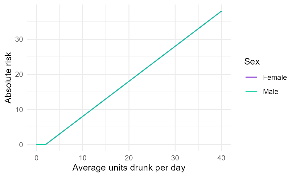
Figure 1. Illustrative linear absolute risk function for a wholly-attributable chronic harm. It is assumed that people are not at risk of harm unless they drink to levels above the UK health drinking guidelines of 2 units/day on average (14 units/week). Above these thresholds, it is assumed that risk increases linearly with the amount drunk.
Implementing in the STAPM code
The SAPM method is implemented unchanged in the STAPM code, within
the function tobalcepi::RRalc().
Acute diseases wholly attributable to alcohol
Here we describe the approach taken in STAPM to model the health harms that are wholly-attributable to level of acute alcohol intake on a single occasion. The health harms that we consider in this category are conditions associated with the effects of excessive blood level of alcohol, toxic effects of alcohol, alcohol poisoning, and acute intoxication. “Wholly-attributable acute” means that these conditions cannot occur without alcohol (i.e. all cases are due to alcohol consumption) and the risk of these conditions changes with acute exposure to alcohol.
The SAPM method
We build on the method used to model the acute health harms that are wholly-attributable to alcohol in the Sheffield Alcohol Policy Model (SAPM).
The main issue to be overcome in the development of SAPM was that there was no available evidence on the relationship between the level of acute exposure to alcohol within a single drinking occasion and the risk of acute harms that were wholly attributable to this acute exposure. Assumptions therefore needed to be made about the shape of the risk function that links the level of single occasion drinking to the risk of acute harms (the approach taken is described on page 29 in the Purshouse et al. modelling report for NICE (2009)).
In addition, due to the harms being wholly-attributable to alcohol, no cases are expected in people who consume below a certain threshold of alcohol on a single occasion, i.e. there are no cases in the non-exposed reference group. One of the consequences of this is that it is not possible to calculate relative risk; instead, the relationship between single occasion drinking and acute harm must be represented by an absolute risk function, e.g. in terms of the expected number of deaths or hospitalisations if a certain number of people were to drink a certain number of units of alcohol on a single occasion. Figure 1 shows the shape of the risk function currently used in SAPM.
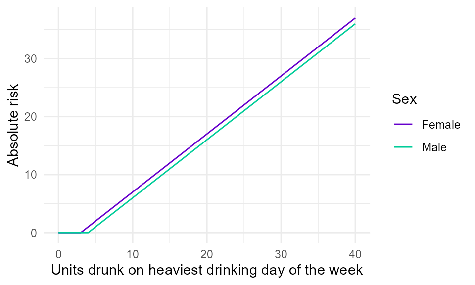
Figure 1. Illustrative linear absolute risk function for a wholly-attributable acute harm. It is assumed that males are not at risk of acute harm unless they drink over 4 units on a single occassion, and that females are not at risk unless they drink over 3 units on a single ocassion. Above these thresholds, it is assumed that risk increases linearly with the amount drunk. SAPM uses data from the Health Survey for England on the amount drunk on the heaviest drinking day in the last 7 days.
Adaptation to suit STAPM
The problem
The main difference between SAPM and STAPM is that STAPM simulates the
individual life-course dynamics of the average weekly amount of alcohol
consumed - STAPM does not simulate the dynamics of the amount drunk on
the heaviest drinking day. This means that for STAPM, we need to develop
a method to link the risk of acute harms that are wholly-attributable to
alcohol consumption to average weekly alcohol consumption.
The solution
The solution is to draw on the methods for partially attributable acute
conditions, which uses parameter values from Hill-McManus et al. (2014) to infer the characteristics of
single occasion drinking from average weekly alcohol consumption and a
range of individual-level covariates. Using the method in
tobalcepi::AlcBinge_stapm() we can calculate the average
parameter values by age, sex and IMD quintile. Using these parameter
values, we can translate each individual’s average weekly alcohol
consumption to their expected number of weekly drinking occasions, and
the distribution of the amounts that each individual drinks on their
drinking occasions. For each individual, we can then calculate the total
number of units per year that are drunk after each individual has
already exceeded the single occasion drinking thresholds of 4 units/day
for men and 3 units/day for women.
Implementing in the STAPM code
A new function tobalcepi::WArisk_acute() has been created
to calculate the total number of units that each individual is expected
to drink above the single ocassion binge drinking thresholds. This
function is called from within the function
tobalcepi::RRalc() and uses the parameters outputs by
tobalcepi::AlcBinge_stapm().
Lag times between changes in alcohol consumption and disease risk
All lag times are taken from the review by (Holmes et al. 2012) and are the numbers used in the current version of SAPM.
Tobacco related risks of disease
See the smoking and disease risks report (Webster et al.
2018). The Sheffield Tobacco Policy Model (STPM) considers 52
adult diseases related to smoking and the corresponding relative risks
of developing these diseases in current vs. never smokers, and in former
smokers according to the time since they quit. The first step carried
out by tobalcepi::RRFunc() is to assign both current and
former smokers the relative risk for each disease associated with
current smoking. It does this using the function
tobalcepi::RRTob().
For current smokers, the current version of the modelling assumes
that the relative risks of disease are the same for all smokers
regardless of the amount currently smoked and the length of time as a
smoker, although we have begun to review and incorporate available
dose-response risk functions for smoking (the function
tobalcepi::RRTobDR() estimates each individual in the data
their dose-response relative risk based on the number of cigarettes they
consume per day). STPM is also currently limited to the consideration of
diseases that affect the consumer themselves e.g. excluding secondary
effects of smoking.
We arrived at the list of tobacco related diseases used in STPM through a process of reviewing the diseases considered by previous health economic models of smoking, and reviewing reports and papers that reviewed the disease risks of smoking (Pokhrel et al. 2013; Callum and White 2004; NHS Digital 2018; US Surgeon General 2014; Carter et al. 2015; Tobacco Advisory Group of the Royal College of Physicians 2018; Brown et al. 2018). The STPM disease list was influenced heavily by our involvement in Chapter 2 of the RCP report ‘Hiding in plain sight’ (Tobacco Advisory Group of the Royal College of Physicians 2018). We were further influenced by discussions within our research group relating to updates to the list of diseases related to alcohol, their ICD-10 code definitions and the published sources of relative risk estimates. As part of these discussions for alcohol we made contact with the authors of the CRUK paper (Brown et al. 2018). Discussions focused particularly on the ICD-10 definitions of head and neck cancers, and oesophageal cancers. The result of these discussions was an updated list of alcohol related diseases for the Sheffield Alcohol Policy Model (SAPM) v4.0 (Angus et al. 2018). In producing our list of smoking related diseases we sought to harmonise our ICD-10 definitions with those used in our alcohol modelling. Our resulting list is mainly consistent with the RCP report, with most deviations being for cancers, where we have been influenced by CRUK’s work and our alcohol modelling. We explain the choices we made in the report where we initially presented our disease list (Webster et al. 2018).
The notable omissions from our list are:
-
Breast cancer—due to a small and statistically uncertain
effect of smoking;
-
Prostate cancer—due to a lack of published evidence for
current smokers;
- Ovarian cancer—for which smoking only carries a risk for fully malignant mucinous ovarian cancers (13% of ovarian cancers are mucinous, and of these 57% are fully malignant), which made it difficult to identify the cases attributable to smoking using the ICD-10 definitions recorded in mortality and hospital episode data.
For oesophageal cancer, our discussions with CRUK concluded that we should distinguish between adenocarcinoma (AC) and squamous cell carcinoma (SCC). However, it is not possible to distinguish these subtypes from the routinely recorded ICD-10 codes. We therefore settled on the following approach: We apportion overall oesophageal cancer prevalence between AC and SCC using estimates of percentage prevalence by age and sex shared with us by CRUK; these data are for 2014 for England and derive from UK cancer registry on the number of oesophageal SCCs.
Risk in former smokers
To estimate the risk of disease for former smokers we used the findings of Kontis et al. (2014), who re-analysed the change in risk after smoking in the ACS-CPS II study from Oza et al.(2011). Since Kontis et al. only provide estimates for cancers, CVD or COPD, we had to decide how to specify the rates of decline in the risks due to smoking after quitting for other diseases. Kontis et al. (2014) consider this issue for type II diabetes, stating that “Randomised trials also indicate that the benefits of behaviour change and pharmacological treatment on diabetes risk occur within a few years, more similar to the CVDs than cancers (Knowler et al. 2002). Therefore, we used the CVD curve for diabetes.” In-line with Kontis et al. (2014), we apply the rate of decline in risk of CVD after quitting smoking to type II diabetes.
We had to make further assumptions about how the risk due to smoking declines after quitting for other diseases (these assumptions are under review and their influence on model findings can be tested with sensitivity analyses). Our default is to assume that the decline in risk for all respiratory conditions follows Kontis et al.’s (2014) estimates for COPD. For other diseases, we might assume that the decline in relative risk follows the cancer curve (the slowest decline in risk), that the additional risk from smoking disappears immediately following quitting (the fastest decline in risk), or that the risk immediately falls to the average risk in former smokers identified from meta-analyses (potentially a middle-ground option, although these estimates will be influenced by differences in study design e.g. in average length of follow-up). The default option in the current version of STPM is to apply the most conservative option that the decline in risk for other diseases follows the cancer curve.
To estimate the risk of disease in former smokers, they are initially assigned the relative risk for each disease associated with current smoking. This risk is then scaled downwards according to the time since quitting, using the equation
\[\begin{equation} RR_{former}=1+[RR_{current}-1][1-p(f)], \end{equation}\]
in which the relative risk (\(RR\)) associated with current smoking is scaled according to our estimates of the proportional reduction in the risk (\(p\)) associated with their number of years (\(f\)) as a former smoker. After someone has been quit for 40 years, we assume their risk reverts back to be the same as a never smoker.
Tobacco–Alcohol interactions in disease risk
When we talk about tobacco-alcohol interactions in disease risk, what we mean is that we want to account for any additional increase in risk of disease that occurs for people who both smoke and drink alcohol. See VanderWeele and Knol (2014) for an explanation of measures of interaction. The rationale for considering this risk interaction is that for some diseases there can be physiological interactions between substances in alcoholic beverages and in tobacco smoke that mean that when both alcohol and tobacco are consumed, then the disease-causing effect of either one is greater.
In 2015, we conducted a scoping review across all diseases for which tobacco and alcohol are causal factors to ascertain the extent of evidence on interaction effects. We included only interactions with a meta-analysis of effect size. The only diseases for which we found suitable meta-analyses to inform the tobacco–alcohol interaction in risk was cancers of the oral cavity, pharynx, larynx (for which we used estimated of head and neck cancer overall: alcohol alone 1.06, tobacco alone 2.37, tobacco and alcohol 5.73) (Hashibe et al. 2009), and Squamous Cell Carcinoma (SCC) of the oesophagus (alcohol alone 1.21, tobacco alone 1.36, alcohol and tobacco 3.28) (Prabhu, Obi, and Rubenstein 2014). Interactions estimated from odds ratios were assumed to be equivalent to interactions estimated from relative risks.
Prabhu et al. (2014) reported interaction effects using a metric of multiplicative interaction called the “Synergy Factor”. The Synergy Factor gives the factor by which the relative risk of disease in someone who both smokes and drinks (\(RR_{ta}\)) exceeds the product of the relative risks in someone who only smokes (\(RR_{t}\)) and someone who only drinks (\(RR_{a}\)):
\[\begin{equation} \text{Synergy Factor} = \frac{RR_{ta}}{RR_t \times RR_a}. \end{equation}\]
In the STAPM modelling, interaction estimates from the literature are applied on the additive rather than multiplicative scale by estimating a metric called the “Synergy Index” (Rothman 1986.). The Synergy Index measures the extent to which the relative risk for someone who both smokes and drinks exceeds 1, and whether this is greater than the sum of the extent to which the relative risk of people who only smoke or only drink exceeds 1:
\[\begin{equation} \text{Synergy Index} = \frac{RR_{ta}-1}{(RR_t-1)+(RR_a-1)}. \end{equation}\]
For head and neck cancer overall, the Synergy Index is estimated to be 3.09, and for oesophageal SCC the Synergy Index is 1.99.
Data on the synergistic effects of tobacco and alcohol risks are
stored in the package repository in the spreadsheet
tobalcepi/vignettes/inst/tob_alc_interactions_180119.csv
and as package data in
tobalctobalcepi::tob_alc_risk_int.
The interaction effects are applied in the STAPM modelling using the
functions tobalcepi::RRFunc() and
tobalcepi::TobAlcInt(). The function
tobalcepi::TobAlcInt() contains code that calculates the
Synergy Index according to the above formula. The function
tobalcepi::RRFunc() then combines the relative risks for
diseases that are related to both tobacco and alcohol using the additive
scale formula:
\[\begin{equation} RR_{ta} = 1 + \left[\left((RR_a - 1) + (RR_t - 1)\right) \times \text{Synergy Index}\right]. \end{equation}\]